Activity 7: Enhancement in the Frequency Domain

A. Anamorphic Property of Fourier Transform

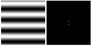
Using the codes below, a 2D sinusoid was created and its Fourier Transform(FT) was shown.

nx = 100; ny = 100;
x = linspace(-1,1,nx);
y = linspace(-1,1,ny);
[X,Y] = ndgrid(x,y);
f = 4 //frequency
z = sin(2*%pi*f*X);
scf(1);
imshow(z,[]);
fftz = fft2(z);
scf(2);
imshow (abs(fftz), []); // FT modulus

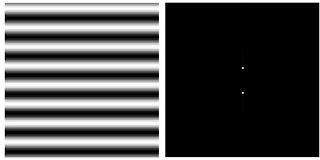
The following images have frequencies of 2, 4 and 24. It can be observed that as the
frequency is increased the farther the points are from each other.





//Rotation
theta = 30;
z1 = sin(2*%pi*f*(Y*sin(theta) + X*cos(theta)));
fftz1 = fft2(z1);
scf(3);
imshow (abs(fftz1), []);

The following were rotated at 30, 45, and 60 degrees. The FT of the image is tilted just like
the original image is.
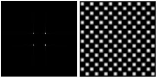
//combination
z2 = sin(2*%pi*4*X).*sin(2*%pi*4*Y);
fftz2 = fft2(z2);
scf(4);
imshow (abs(fftz2), []);


B. Ridge enhancement
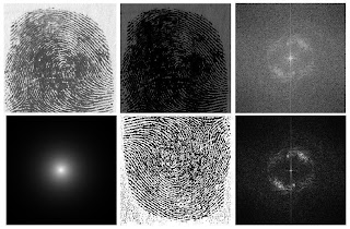
Using the code below, the fingerprint was enhanced. This was done by using a high pass filter.
img = imread('C:\Users\nez\Desktop\activity 7 final\finger.jpg');
imgray = im2gray(img);
pic =imgray-mean(img);
scf(1);
imshow(pic);

im=fft2(pic);

ff=real((im).*conj(im));
scf(3);
imshow(fftshift(log(ff+1)),[]);
xset('colormap',jetcolormap(64));

//Transfer function
filter=mkfftfilter(pic,'exp',30);
scf(4);
imshow(filter);

//High-pass filter
IM=im.*fftshift(1-filter);
IMAGE=real(fft2(IM));
scf(5); imshow(IMAGE);

scf(6);
imshow(abs(fftshift(fft2(IMAGE))), []);
xset('colormap', jetcolormap(64));


(clockwise from top left: original image; mean centered image; FFT of mean centered image; FFT of enhanced image; enhance image; filter)


C. Line Removal

This was done using the code below. A filter was used to remove the lines from the original image.
img = imread("C:\Users\nez\Desktop\activity 7 final\hi_res_vertical_lg.gif");
imgray = im2gray(im);
Fimgray = fft2(imgray);

scf(1);
imshow(fftshift(abs(Fimgray)),[]);

//filtering
b = imread('C:\Users\nez\Desktop\activity 7 final\filter2.bmp');
a = imread('C:\Users\nez\Desktop\activity 7 final\hi_res_vertical_lg.gif');

bgray = im2gray(b);
agray = im2gray (a);
Fb = fftshift(bgray);
Fa = fft2 (agray);
FRA = Fb.*(Fa);
IRA = fft2 (FRA); //inverse FFT
FImage = abs(IRA);
imshow(FImage, [ ]);

Grade: 6/10 - It was passed late.

Activity 6: FOurier Transform of Image Model

*Familiarization with discrete FFT

smallest_circle

circle

smaller circle Image above(clockwise from top left): original image; FFT of image; shifted FFT of image; original image with FFT applied twice.

Using the code below resulted to the images above. When FFT is applied twice to an image, an image of the original image is produced. This maybe so for a centered circle but the difference can clearly be seen when the same procedure is done to an image not centered and non-uniform in shape. (Note: circle produced after applying FFT twice is a bit out of shape because it was scaled.)

I = imread('circle.bmp');
Igray = im2gray(I);
FIgray = fft2(Igray); //FIgray is complex
scf(1);

imshow(abs(FIgray),[]);

scf(2);

imshow(fftshift(abs(FIgray))), []);

scf(3);

imshow(abs(fft2(fft2(I))));

The code above was again used, and this time, the image of the letter A is now inverted after applying FFT twice. This happens because when FFT is used, the quadrants along the diagonals interchange.

Image above(clockwise from top left): original image, FFT of image; image after applying FFT twice; shifted FFT of image.(The inverted image was scaled .)

*Simulation of an imaging device

r=imread('C:\MyDocuments\AP186\circle.bmp');
a=imread('C:\MyDocuments\AP186\VIP.bmp');
rgray = im2gray(r);
agray = im2gray(a);
Fr = fftshift(rgray);//aperture is already in the Fourier Plane and need not be FFT'ed
Fa = fft2(agray);
FRA = Fr.*(Fa);
IRA = fft2(FRA); //inverse FFT
FImage = abs(IRA);
imshow(FImage, [ ]);

Using this code, the following images were produced:

Image above(clockwise from top left): original image; convolved image using circle image; convolved image using smaller_circle image; convolved image using smallest_circle image.



As we can see, as the circle being used gets smaller, the quality of the image becomes lesser.



*Template matching using correlation


r=imread('C:\MyDocuments\AP186\text.bmp');


a=imread('C:\MyDocuments\AP186\A.bmp');


rgray = im2gray(r);


agray = im2gray(a);


Fr = fftt2(rgray);


Fa = fft2(agray);

b = conj(Fr);
FRA = (Fa).*b;


IRA = fft2(FRA);


FImage= abs(IRA);


imshow(FImage, [ ]);

With this code, the originial image became unrecognizable. The texts in the image looked like letters A.

*Edge detection using convolution integral

pattern = [-1 -1 -1; 2 2 2; -1 -1 -1];

a=imread('C:\MyDocuments\AP186\VIP.bmp');
image = imcorrcoef(a, pattern);
imshow (image, []);

Using the code, the following images were formed. The first image shows a horizontal pattern since the pattern used here is also horizontal. The second image used a vertical pattern hence the image of VIP followed that pattern. It's also the same with the 3rd image, this time a spot pattern was used.

Acknowledgements: Jorge Presto

Grade: 10/10 - because the activity was well done.

Activity 5

The code for getting the Fourier transform of a signal is given below:
//Generate 1-D sinusoid of form sin(2*pif*t)

T = 2;//total time interval
N = 256;//number of samples
dt = T/N;//sampling interval
t = [0:dt:(N-1)*dt];
f = 5;//frequency
y = sin(2*%pi*f*t);
f1 = scf(1); plot(t,y);

//FT of the signal and computation of frequency scale.
FY = fft(y);
F = 1/(2*dt);//max frequency
df = 2*F/256;//discrete frequency
f = [-(df*(N/2)):df:df*(N/2 -1)];

//shifted FFT output with frequency axis
f2 = scf(2);

plot(f, fftshift(abs(FY)));

Using this code results to the images below which shows the sinusoidal signal and the plot of the Fourier transform of the signal.

T=256; N =2

Answers to questions:

4. In the case of images, 2-D Discrete Fourier Transform(DFT) will be used and is given by the formula:

Applying DFT will decompose the image to its sinusoidal components. Note that the Image should be in grayscale.

5.

a) The threshold sampling interval can be found by using the formula:

Fmax = 1/(2*dT)
where Fmax is equal to 120 Hz and dT is the threshold sampling interval.
This results to a thresholding sampling interval equal to 0.0041667

b) Increasing the number of samples N results to a higher peak as shown below.
N = 512; T = 4

c) Decreasing sampling interval dt results to a smaller interval between the peaks.
N = 256; T = 1
d) Increasing the number of samples N while fixing the total time interval T results to a higher peak but interval between them is the same with the original.
N =512; T = 2
Acknowledgement: Jorge Presto

Grade: 10/10 - Activity was done and questions were all answered.