Sunday, October 12, 2008

A15: Color Image Processing

In this activity, two popular algorithms will be used for white balancing. The Reference White Algorithm(RWA) and the Gray World Algorithm(GWA). For RWA, we will pick a color in an image as reference for white. Its RGB values will then be used to divide other RGB channels. For GWA, we take the average of each channel and take their averages as balancing constants. 

Using these algorithms, we compare the images after application to different white balance settings of the camera. 

Flourescent


Tungsten


Daylight


Blue objects


Comparing the images from both algorithms, the reference white is much better to use than the gray world algorithm in images where there are many colors. The same goes for images with just different hues.

CODE:

//Reference White

I = imread('image');

imshow(I);

pix = locate(1);

Rw = I(pix(1), pix(2), 1);

Gw = I(pix(1), pix(2), 2);

Bw = I(pix(1), pix(2), 3);


I(:, :, 1) = I(:, :, 1)/Rw;

I(:, :, 2) = I(:, :, 2)/Gw;

I(:, :, 3) = I(:, :, 3)/Bw;

I(I > 1.0) = 1.0;

imshow (I);


//Gray World

I = imread('image');

Rw = mean(I(:, :, 1));

Gw = mean(I(:, :, 2));

Bw = mean(I(:, :, 3));


I(:, :, 1) = I(:, :, 1)/Rw;

I(:, :, 2) = I(:, :, 2)/Gw;

I(:, :, 3) = I(:, :, 3)/Bw;

I = I * 0.5;

imshow(I);

A17: Basic Video Processing

This activity shows basic video processing. Using a video of an ink diffusing in water, the are of the ink in the diffused water was determined.


Video of Ink Diffusion

Cropping the video so that only the area of diffusion can be viewed, the video was converted to many frames of still images. With this images, the threshold was determined using GIMP and then the images were binarized for area estimation.


Through pixel counting, the results are showed in the graph below on the left. Comparing this with the theoretical values in figure 5 from Lee S., et al, 2004,we can see that there are errors in our data. This is due to the pixel counting method. Not all of the images that were pixel counted are ink.


Wednesday, August 13, 2008

Activity 13: Photometric Stereo

By capturing multiple images of a surface with light sources at different locations. In this activity, the images used are the following below.


To do this, N sources in 3D space are defined in matrix form

Since I = Vg, we can solve for the surface normal. I is the intensity matrix and V is matrix form for the sources. To get surface normal, we use the equations


With the surface normals determined, the elevation is the computed and plotted in 3D space.


loadmatfile ('C:\Users\nez\Documents\tresloco\ap186_2\activity13\Photos');
browsevar();
I(1,:) = (I1(:))';
I(2,:) = (I2(:))';
I(3,:) = (I3(:))';
I(4,:) = (I4(:))';
V(1,:) = [0.085832 0.17365 0.98106];
V(2,:) = [0.085832 -0.17365 0.98106];
V(3,:) = [0.17365 0 0.98481];
V(4,:) = [0.16318 -0.34202 0.92542];
g = (inv(V'*V)*(V'))*I;
N = size(g);gmag = [];
for i = 1:N(2)
gmag(i) = sqrt(g(1,i)**2 + g(2,i)**2 + g(3,i)**3)+0.0000000001;
end

n(1,:) = g(1,:)./gmag(1,:);
n(2,:) = g(2,:)./gmag(1,:);
n(3,:) = g(3,:)./gmag(1,:);
dfx = -n(1,:)./(n(3,:)+0.0000000001);
dfy = -n(2,:)./(n(3,:)+0.0000000001);

F = cumsum(dfx,1)+cumsum(dfy,2);
new = matrix(F,[128,128]);
plot3d(1:128,1:128,new)
Using this code, a 3D plot of the suface was created.

Grade: 8/10 - I have done the activity well.

Monday, August 11, 2008

Activity 11: Camera Calibration


The activity was done using the image below.


Letting the origin be at the lowest part of the board along the middle, coordinates of 20 corner points were measured. Using Microsoft Paint, the coordinates for each picked corner in the image was determined.


x0 = [0 1 3 0 2 0 0 0 8 3 0 0 0 0 3 8 5 1 6 0];
y0 = [0 0 0 3 0 6 7 3 0 0 8 1 6 8 0 0 0 0 0 2];
z0 = [0 1 4 5 9 11 5 7 0 12 7 10 9 0 6 8 8 10 11 1];
yi = [100 117 154 70 138 37 24 70 243 157 13 92 36 13 154 248 192 120 212 80];
zi = [234 218 163 145 62 26 156 105 251 3 115 41 68 265 123 89 86 41 26 222];for i = 1:20
Q((2*i)+1,:) = [x0(i) y0(i) z0(i) 1 0 0 0 0 -(yi(i)*x0(i)) -(yi(i)*y0(i)) -(yi(i)*z0(i))];
Q((2*i)+2,:) = [0 0 0 0 x0(i) y0(i) z0(i) 1 -(zi(i)*x0(i)) -(zi(i)*y0(i)) -(zi(i)*z0(i))];
d((2*i)+1,:) = [yi(i)];
d((2*i)+2,:) = [zi(i)];
end
Qt = Q'
a = inv(Qt*Q)*Qt*d;


//check
for j = 1:20
y2(j,:) = ((a(1))*x0(j)+(a(2))*y0(j)+(a(3))*z0(j)+a(4))/((a(9))*x0(j)+(a(10))*y0(j)+(a(11))*z0(j)+1);
z2(j,:) = ((a(5))*x0(j)+(a(6))*y0(j)+(a(7))*z0(j)+a(8))/((a(9))*x0(j)+(a(10))*y0(j)+(a(11))*z0(j)+1);
end
The code above used the equation from the manual.


The result was having an average % error of 0.7947295 and 1.245960579 in y and z respectively.


//verification for other points

x0 = [3 7 0];

y0 = [0 0 2];

z0 = [5 2 7];

for k = 1:3

y3(k,:) = ((a(1))*x0(k)+(a(2))*y0(k)+(a(3))*z0(k)+a(4))/((a(9))*x0(k)+(a(10))*y0(k)+(a(11))*z0(k)+1);

z3(k,:) = ((a(5))*x0(k)+(a(6))*y0(k)+(a(7))*z0(k)+a(8))/((a(9))*x0(k)+(a(10))*y0(k)+(a(11))*z0(k)+1);
end
The results show that the method was accurate.
Grade: 7/10 - The activity was passed late.
Acknowledgement: Jorge Presto

Activity 10: Preprocessing Handwritten Text


After cropping a portion from the image above, the new image's Fourier Transform was determined.
im=imread('C:\Users\nez\Documents\tresloco\ap186_2\activity 10\a.jpg');
img = im2gray(im);
imgfft=fft2(img);
scf (1);
imshow(imgfft);
imwrite (imgfft, 'C:\Users\nez\Documents\tresloco\ap186_2\activity 10\imgray.jpg')

With the use of techniques learned from previous activities, the lines were removed using a filter just like the one below.

filter=imread('C:\Users\nez\Documents\tresloco\ap186_2\activity 10\f.jpg');

imf = im2gray(filter);

imffft=fftshift(imf);

imffft=ff1.*ff2; The image is then convolved with the filter, converted to binary, and cleaned using the closing/opening operator.

//filtering the image

a=real(fft2(imffft));

scf(2)imshow(a,[]);

imwrite (a, 'C:\Users\nez\Documents\tresloco\ap186_2\activity 10\imfilter.jpg')

//binarize the image

b=im2bw(a, 127/255);

c=1-b;

scf(3);imshow(c,[]);

imwrite (c, 'C:\Users\nez\Documents\tresloco\ap186_2\activity 10\imbinary.jpg')

//opening operation

SE = ones(2,2);

d=erode(c,SE);

e=dilate(d,SE)scf(4);

imshow(e,[]);

imwrite (e, 'C:\Users\nez\Documents\tresloco\ap186_2\activity 10\imcloseopen.jpg')


After this is done, the image is then labelled.
//labelling the image
imfinal=bwlabel(e);
scf(5);
imshow(imfinal,[]);
//imwrite (imfinal, 'C:\Users\nez\Documents\tresloco\ap186_2\activity 10\imlabel.jpg')


Grade: 6/10 - I passed it too late.
Acknowledgement: Jorge Presto

Activity 9 :Binary Operations

The activity's objective is to find the best estimate of the cell area. Using GIMP, the image above was cropped into 9 parts measuring 256 x 256 pixels. The subimages were then converted to black & white by finding the threshold of the images.
With the code below, the closing and opening operators were used to clean the image of isolated pixels andcells very near each other.
//img = imread("G:\to be posted\186_09\C1_01_bw.jpg");

//img = imread("G:\to be posted\186_09\C1_02_thresh205.jpg");
//img = imread ("G:\to be posted\186_09\C1_03_thresh223.jpg");
//img = imread ("G:\to be posted\186_09\C1_04_thresh194.jpg");
//img = imread ("G:\to be posted\186_09\C1_05_thresh190.jpg");
//img = imread ("G:\to be posted\186_09\C1_06_thresh215.jpg");
//img = imread ("G:\to be posted\186_09\C1_07_thresh200.jpg");
//img = imread ("G:\to be posted\186_09\C1_08_thresh194.jpg");
img = imread ("G:\to be posted\186_09\C1_09_thresh213.jpg");
imgray = im2gray(img);
mat = size(img);
pic = imgray;for i = 1:mat(1) //rows
for j = 1:mat(2) //columns
if pic(i,j) <>
pic(i,j) = 0;
else
pic(i,j) = 1;
end
end
end

SE = [];for i = 1:4 for j =1:4 SE(i,j) = 1; end end
img_co = erode(dilate(pic,SE),SE);

//img_co = dilate(erode(pic,SE),SE);
scf(1);
imshow (img_co4);
imwrite (img_co4, 'G:\to be posted\186_09\C1_09_co.jpg');

After cleaning the images, each blob was then labelled and the area of each was measured.

//labellingimg = imread ("G:\to be posted\186_09\C1_09_co.jpg");
imgray = im2gray (img);pic = imgray;
mat = size(pic);
for x = 1:mat(1);
for y = 1:mat(2);
if pic (x, y) <>
pic (x, y) = 0;
else
pic (x, y) = 1;
end
end
end[L, n] = bwlabel(pic);
scf(3);
imshow(pic, []);
scf(4);
imshow (L+1,rand(n+1,3));

//area
for i = 1: max(bwlabel(pic))
v = find(L == i);
w = size(v);
area(i) = w(2);
end

The following images show the blobs binarized, cleaned, and labelled.


With the use of Microsoft Excel, the histogram was plotted. The values used were in the range of 400 to 700. mean = 498.2 ; standard deviation = 55.19

Wednesday, July 23, 2008

Activity 7: Enhancement in the Frequency Domain

A. Anamorphic Property of Fourier Transform

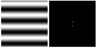
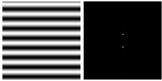
Using the codes below, a 2D sinusoid was created and its Fourier Transform(FT) was shown.

nx = 100; ny = 100;
x = linspace(-1,1,nx);
y = linspace(-1,1,ny);
[X,Y] = ndgrid(x,y);
f = 4 //frequency
z = sin(2*%pi*f*X);
scf(1);
imshow(z,[]);
fftz = fft2(z);
scf(2);
imshow (abs(fftz), []); // FT modulus

The following images have frequencies of 2, 4 and 24. It can be observed that as the
frequency is increased the farther the points are from each other.


//Rotation
theta = 30;
z1 = sin(2*%pi*f*(Y*sin(theta) + X*cos(theta)));
fftz1 = fft2(z1);
scf(3);
imshow (abs(fftz1), []);

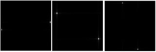
The following were rotated at 30, 45, and 60 degrees. The FT of the image is tilted just like
the original image is.
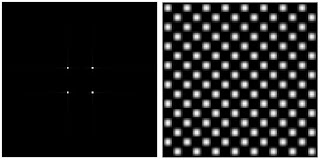
//combination
z2 = sin(2*%pi*4*X).*sin(2*%pi*4*Y);
fftz2 = fft2(z2);
scf(4);
imshow (abs(fftz2), []);


B. Ridge enhancement
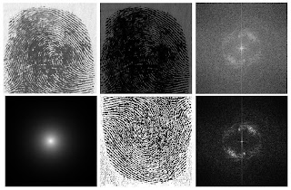
Using the code below, the fingerprint was enhanced. This was done by using a high pass filter.
img = imread('C:\Users\nez\Desktop\activity 7 final\finger.jpg');
imgray = im2gray(img);
pic =imgray-mean(img);
scf(1);
imshow(pic);

im=fft2(pic);

ff=real((im).*conj(im));
scf(3);
imshow(fftshift(log(ff+1)),[]);
xset('colormap',jetcolormap(64));

//Transfer function
filter=mkfftfilter(pic,'exp',30);
scf(4);
imshow(filter);

//High-pass filter
IM=im.*fftshift(1-filter);
IMAGE=real(fft2(IM));
scf(5); imshow(IMAGE);

scf(6);
imshow(abs(fftshift(fft2(IMAGE))), []);
xset('colormap', jetcolormap(64));


(clockwise from top left: original image; mean centered image; FFT of mean centered image; FFT of enhanced image; enhance image; filter)


C. Line Removal

This was done using the code below. A filter was used to remove the lines from the original image.
img = imread("C:\Users\nez\Desktop\activity 7 final\hi_res_vertical_lg.gif");
imgray = im2gray(im);
Fimgray = fft2(imgray);

scf(1);
imshow(fftshift(abs(Fimgray)),[]);

//filtering
b = imread('C:\Users\nez\Desktop\activity 7 final\filter2.bmp');
a = imread('C:\Users\nez\Desktop\activity 7 final\hi_res_vertical_lg.gif');

bgray = im2gray(b);
agray = im2gray (a);
Fb = fftshift(bgray);
Fa = fft2 (agray);
FRA = Fb.*(Fa);
IRA = fft2 (FRA); //inverse FFT
FImage = abs(IRA);
imshow(FImage, [ ]);

Grade: 6/10 - It was passed late.

Monday, July 7, 2008

Activity 6: FOurier Transform of Image Model


*Familiarization with discrete FFT


smallest_circle


circle

smaller circle Image above(clockwise from top left): original image; FFT of image; shifted FFT of image; original image with FFT applied twice.


Using the code below resulted to the images above. When FFT is applied twice to an image, an image of the original image is produced. This maybe so for a centered circle but the difference can clearly be seen when the same procedure is done to an image not centered and non-uniform in shape. (Note: circle produced after applying FFT twice is a bit out of shape because it was scaled.)


I = imread('circle.bmp');
Igray = im2gray(I);
FIgray = fft2(Igray); //FIgray is complex
scf(1);

imshow(abs(FIgray),[]);

scf(2);

imshow(fftshift(abs(FIgray))), []);

scf(3);

imshow(abs(fft2(fft2(I))));


The code above was again used, and this time, the image of the letter A is now inverted after applying FFT twice. This happens because when FFT is used, the quadrants along the diagonals interchange.


Image above(clockwise from top left): original image, FFT of image; image after applying FFT twice; shifted FFT of image.(The inverted image was scaled .)


*Simulation of an imaging device


r=imread('C:\MyDocuments\AP186\circle.bmp');
a=imread('C:\MyDocuments\AP186\VIP.bmp');
rgray = im2gray(r);
agray = im2gray(a);
Fr = fftshift(rgray);//aperture is already in the Fourier Plane and need not be FFT'ed
Fa = fft2(agray);
FRA = Fr.*(Fa);
IRA = fft2(FRA); //inverse FFT
FImage = abs(IRA);
imshow(FImage, [ ]);


Using this code, the following images were produced:


Image above(clockwise from top left): original image; convolved image using circle image; convolved image using smaller_circle image; convolved image using smallest_circle image.


As we can see, as the circle being used gets smaller, the quality of the image becomes lesser.


*Template matching using correlation


r=imread('C:\MyDocuments\AP186\text.bmp');


a=imread('C:\MyDocuments\AP186\A.bmp');


rgray = im2gray(r);


agray = im2gray(a);


Fr = fftt2(rgray);


Fa = fft2(agray);

b = conj(Fr);
FRA = (Fa).*b;


IRA = fft2(FRA);


FImage= abs(IRA);


imshow(FImage, [ ]);

With this code, the originial image became unrecognizable. The texts in the image looked like letters A.

*Edge detection using convolution integral


pattern = [-1 -1 -1; 2 2 2; -1 -1 -1];

a=imread('C:\MyDocuments\AP186\VIP.bmp');
image = imcorrcoef(a, pattern);
imshow (image, []);

Using the code, the following images were formed. The first image shows a horizontal pattern since the pattern used here is also horizontal. The second image used a vertical pattern hence the image of VIP followed that pattern. It's also the same with the 3rd image, this time a spot pattern was used.

Acknowledgements: Jorge Presto

Grade: 10/10 - because the activity was well done.

Wednesday, July 2, 2008

Activity 5


The code for getting the Fourier transform of a signal is given below:
//Generate 1-D sinusoid of form sin(2*pif*t)
T = 2;//total time interval
N = 256;//number of samples
dt = T/N;//sampling interval
t = [0:dt:(N-1)*dt];
f = 5;//frequency
y = sin(2*%pi*f*t);
f1 = scf(1); plot(t,y);

//FT of the signal and computation of frequency scale.
FY = fft(y);
F = 1/(2*dt);//max frequency
df = 2*F/256;//discrete frequency
f = [-(df*(N/2)):df:df*(N/2 -1)];

//shifted FFT output with frequency axis
f2 = scf(2);
plot(f, fftshift(abs(FY)));

Using this code results to the images below which shows the sinusoidal signal and the plot of the Fourier transform of the signal.


T=256; N =2


Answers to questions:


4. In the case of images, 2-D Discrete Fourier Transform(DFT) will be used and is given by the formula:


Applying DFT will decompose the image to its sinusoidal components. Note that the Image should be in grayscale.


5.


a) The threshold sampling interval can be found by using the formula:

Fmax = 1/(2*dT)
where Fmax is equal to 120 Hz and dT is the threshold sampling interval.
This results to a thresholding sampling interval equal to 0.0041667

b) Increasing the number of samples N results to a higher peak as shown below.
N = 512; T = 4


c) Decreasing sampling interval dt results to a smaller interval between the peaks.
N = 256; T = 1
d) Increasing the number of samples N while fixing the total time interval T results to a higher peak but interval between them is the same with the original.
N =512; T = 2
Acknowledgement: Jorge Presto

Grade: 10/10 - Activity was done and questions were all answered.

Wednesday, June 18, 2008

Area Estimation for Images with defined edges

The shapes that were measured were that of a circle, triangle, and square. Using scilab and the green's theorem, the following were acquired:
shape - area(pixel count) - Area - percent error
square - 27225 - 26993.5 - 0.850
triangle - 13622 - 13493 - 0.947
circle - 29757 - 29532 - 0.756


I give myself a grade of 8, since the percent errors were minimal but I was helped and guided by Ed David and Jorge Presto.

Wednesday, June 11, 2008

Activity 1

After counting the number of pixels in each division in the x and y axis, I used ratio and proportion. Using those results I plotted the points of the graph using excel.

I give myself a grade of 9. This is because the graph generated from microsoft excel did not exactly match that of the original image.